Understanding Characteristic Impedance, VSWR and Reflection Coefficient
by DS Instruments Staff
Oct 2013 DS Instruments
Nothing is more fundamental to understanding RF and microwave principles than understanding the concept of characteristic impedance. Whenever we talk about 50-ohm cable or 75-ohm cable we are really saying that its characteristic impedance is 50ohms, 75 ohms, etc. Characteristic Impedance is usually explained with depressingly few words followed by lots of equations and mathematical arguments. This paper is an attempt to explain it in more intuitive terms.
Its important to realize that the 50 or 75 ohm systems typically used in today’s RF/microwave systems is a “human made” arbitrary choice. It could have easily been 43 ohms or other numbers, but physical size considerations do dictate the range of practical coax cables to be in the 20 to 200 ohm range. The combination of physical size issues on practical coax impedance range and the desire for easy arithmetic gives us the values of characteristic impedance seen today of 50 and 75 ohms(typically).
Just as important is to remember that the characteristic impedance concept is so broad as to include all types of coaxial lines, printed circuit traces, micro-strip, strip-line, twin lead and twisted pair. In fact if your designing PCB transmission lines you can chose the characteristic impedance to be what you want it to be, not just 50 or 75 ohms.
Remarkably even free space itself has characteristic impedance. In the case of free space and other unbounded medium this impedance is called the intrinsic impedance.
An Experiment using some 50-Ohm Coax Cable
Lets say someone hands you a 1000 foot roll of coax cable and says to you ” that is 50 ohm coax use it wisely”. You decide to check out this “50 Ohm” assertion by using your ohmmeter. You connect one lead of the ohmmeter to center conductor the other to outer conductor at one end of the cable. The other end of the cable is left open. You are surprised to see it reads near infinite impedance! Why doesn’t it read 50ohms you wonder? Then you then short the inner conductor to outer conductor at the far end and again measure the open end of the cable with the meter. It now reads near zero ohms! ” How can this be!” you ask yourself, “I was assured it was 50 ohm cable!”
The reason your meter did not tell you that the cable was 50 ohms is that it could NOT read the Instantaneous voltage/current ratio( V=IR). Common ohmmeters have very high internal resistance. Any capacitance in the ohmmeter will combine with the internal resistance to form a very large time constant. This large time constant makes it impossible for this type of instrument to respond fast enough to “see” the high speed pulse you introduced on the coax line the moment you connected the ohmmeter leads to it.
You cannot use a typical ohmmeter to measure characteristic impedance. Instead of trying to use an ohmmeter we will use the circuit of figure 1. The circuit allows us to generate a pulse of current by toggling the switch. The asterisk indicates where wish observe and measure the current.
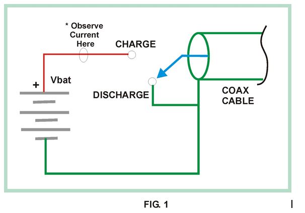
We will assume that the switch has been in the DISCHARGE position for a very long time, ensuring no voltages are present on the coax cable. Now what happens if we were to flip the switch to CHARGE? At the moment the switch connects battery (+) to the center conductor of the coax cable it starts to “charge up” that piece of coax, sort of like charging a capacitor. We could then discharge the cable by shorting center conductor to shield or battery minus or switch in DISCHARGE position.
Thus by operating the simple switch of figure 1 we can introduce a “pulse” of current onto the coax cable. If you measure the current in the center conductor during the moment when the switch is first connected to CHARGE you would see a pulse of current that will reach a maximum value of Imax=Vbat / Zo, where Zo is the characteristic impedance of coax cable. Sometimes the characteristic impedance is called the surge impedance of the coax.
Just what properties of coax limit the inrush current to the expression given above? Or stated another way why doesn’t the coax charge up “instantly”? To answer that question let’s examine the way an ideal capacitor would charge up vs. coax if it were connected to our switch circuit of figure 1.
Charging an Ideal Capacitor with a Battery vs. Ideal Coax
In theory, an ideal, discharged, capacitor would see an infinite current for zero time if you connect it to a perfect source (a perfect voltage source has zero internal resistance). Stated another way the capacitor would charge up “instantly” to the applied voltage of the source. There are two crucial differences in the way a piece of coax charges up and a ideal capacitor would charge up when connected to a battery. First we assumed that an ideal capacitor has zero inductance and zero resistance in the current path. Any non-zero inductance/resistance would limit current inrush rate. Second an ideal capacitor has zero physical length so no there is no propagation in space of the current pulse.
Our piece of coax cable does not charge up instantly. This is so because it does indeed have inductance per lineal foot and it has physical length> 0. Because our piece of coax has a finite series inductance per unit length, a capacitance per unit length and it has a non-zero physical length an applied current pulse will propagate in both time and space.
Specifically the series inductance resists the flow of current that wants to charge the capacitance of the cable. This results in propagation delay of the current surge. This propagation delay causes the current surge to spread out in time, that is its not instantaneous as the in the case of the ideal capacitor. Simultaneously the physical length creates a propagation distribution in space of the current surge. Our current surge travels down the cable from where it started.
Instead of an infinite “impulse” of current in zero time and zero space, as in the ideal capacitor, the coax current quickly rises to a maximum and starts propagating down the coax. The speed of propagation is typically less than the speed of light and depends on the materials the coax is made from, specifically the dielectric constant of the material between inner and outer conductors.
An Equivalent Circuit for a Infinite Length of Coax Cable
From our above discussion we can form an ideal circuit that cannot be distinguished from an ideal infinite length of coaxial cable, see figure 2. By ideal we mean loss-less coax cable and components as well as resistors and capacitors free of parasitic inductance, capacitance and resistance.
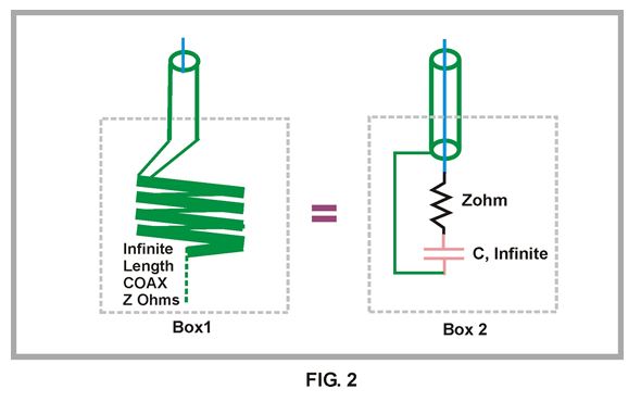
In figure two we have two boxes, 1 and 2. We are not allowed to see inside the boxes all we can see and attach instruments to is 1 foot of exposed coax cable of impedance Z ohm’s. Our task is to determine if the box contains just coax cable or a piece of coax with a circuit attached to it after some amount of cable.
After using ohmmeters, voltmeters, o’scopes, time domain reflectometers, Network Analyzers and anything else we can throw at it, we can see no difference in the measurements and we conclude the two boxes contain the same physical circuit or length of cable.
As shown in figure 2 we can see that they do not. Box 1 contains an infinite length of coax cable and the other box a small section of coax with series RC network attached between the inner conductor and the outer shield at the end of the cable. The series R is equal to the coax cable characteristic impedance Z Ohms and the series capacitor is of infinite capacitance. The purpose of this infinite capacitor is to block DC (but pass all AC) so as to insure that a simple (ideal) ohmmeter check would read infinite resistance, just as it would on the infinite piece of coax in box 1.
In this hypothetical example we had to use ideal components and infinite lengths of cable for our statements to be strictly true. But that does not mean this experiment is not reproducible with real life stuff. In fact with very precise components in Box 2 and a very long piece of high quality coax in Box 1 (>100 miles) it would be very difficult to measure much difference between these two boxes with even with the best of instruments at least over some band of frequencies.
Other ways to Measure Coax Cable Impedance
The current surge method is not how one would normally measure coax cable characteristic impedance but it is a viable method and has an intuitive appeal. Another way to measure the characteristic impedance of coax cable is to measure its inductance and capacitance per unit length; the square root of L divided by C will be in ohms (not farads or henrys) and will be equal to the characteristic impedance.
Why do different cables have different characteristic impedances? Every coax cable or other transmission media has its own unique capacitance and inductance per unit length. For coax cables this will be determined by inner/outer conductor ratios and the dielectric constant of the material between conductors for coax cables. For micro-strip lines it is primarily the trace width, dielectric constant of the pc board and thickness of PC board.
VSWR , One way to Quantify how close we are to ideal Impedance
Perhaps now maybe the “50 Ohm” cable idea makes some sense and you are now a “50 ohm” systems zealot. You now strive for “perfect 50 ohms” in all your cabling, connections and devices. You have become so unreasonable that you insist that all systems be EXACTLY 50 ohms.
Well now you are in trouble. In truth no coax cable, connector, amplifiers etc. is exactly 50 ohms. The fact is that it is amazing how far off 50 Ohms you can be in your designs and not see that much degradation in performance! We need a way of expressing how close we are to 50 Ohms in our designs and systems. The most common way of doing this is what is called VSWR or Voltage Standing Wave Ratio. A complicated sounding name for sure.
It is hoped that with concept of VSWR mastered you will become more reasonable about how close your impedances should be to ideal values. The concept VSWR applies for ANY characteristic impedance, 50 ohms or otherwise.
A piece of Coax and a 50MHz Sine wave Generator
Lets investigate what VSWR is by an example. Suppose you took your 1000-foot roll of 50-ohm coax and cut a 20-foot chunk off it. Now connect one end to the circuit shown in figure 3. In figure 3 the switch and battery of figure 1 have been replaced by a 50-Ohm resistor and a signal source that produces sine waves. We will also assume the generators internal “50 ohms” is perfect in that its always behaves as a resistor with no parasitic inductive or capacitive elements. We will leave the other end of our coax chunk open. We set the sine-wave source frequency to 50 MHz. Although just about any frequency will work, 50 MHz is a good spot for testing most coax.
At this point our circuit of figure 3 is supplying a 50 MHz sine wave into one end of a “50 Ohm” piece of coax with no connection at the other end. What will happen?
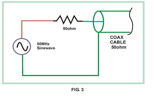
Well here is what happens: The sine wave when FIRST applied to the cable starts to “propagate” towards the open end of the cable, just like our current pulse did. When the sine wave gets to the end of the cable it completely “reflects” , turns around, and heads right back towards the generator! Once inside the generator it “dissipates” itself as heat in the generators internal 50-ohm resistor. Perhaps this is hard to believe but its true**.
Now we repeat the same experiment except we short the other end of the coax cable. Again we would see a complete reflection of the sine wave and total dissipation of reflected wave within the internal 50 ohms of the generator (there will be a phase reversal with respect to OPEN case above).
So, if the cable end is open or shorted we get TOTAL reflection of our applied sine wave. This is defined as a VSWR of “infinity to 1”. Now we connect a “perfect” 50-ohm resistor at the end of the coax line. In this case we have terminated the cable in its characteristic impedance. The applied sine wave will be completely dissipated in this termination and there will be zero reflection. We have fooled the sine wave; it sees our termination as just an “infinite” piece of cable. We have of course come full circle and have arrived again at the equivalent circuit of Box 2 in figure 3 above.
The perfectly terminated condition has the lowest VSWR obtainable and is defined as 1 to 1 or written usually as 1:1. A VSWR of 1:1 for a coax cable termination means it is exactly equal to the characteristic impedance and we will have ZERO reflection from this termination.
Reflection Coefficient, Return Loss and Mismatch Loss
A closely related parameter is the reflection coefficient. This term not only records the magnitude of the reflected wave but also its angle with respect to the source wave. Because the reflection coefficient measures magnitude of reflection and its angle it is VECTOR measurement. VSWR only measures magnitude and is therefore a SCALAR measurement. VSWR can be calculated if the Reflection coefficient is known, see below. The table also shows Return loss and Mismatch loss. Return loss (RL) is a measure of how much power is reflected from a load or termination. The closer the termination or load is to “ideal” characteristic impedance the lower the reflected power. It is expressed in dB referenced to the incident power and is usually negative indicating a lower power reflected than absorbed by load. Again VSWR can be calculated if RL is known. Any RL that is better than -15dB is usually considered quite acceptable.
Mismatch Loss (ML) indicates how much power is lost when a signal (sine wave) travels across a distinct change in characteristic impedance. Since no system of connectors is perfect ML occurs at every connector, connection etc. Okay back to the real world. There are no perfect terminations and there are no perfect 50-ohm resistors. Let’s examine what happens when we use a real world termination on a 50ohm coaxial cable, one that’s slightly off or in some way imperfect.
Connecting a 75Ohm termination to 50Ohm Cable
Suppose you were working on a 50-ohm system and you needed to terminate a open coax cable end to prevent unwanted reflections. Unfortunately the only terminations you have in your pocket are all 75-ohm type. Assuming you can get the connector to mate what will happen if you terminate that 50 ohm line with a 75 ohm termination?
First off 75 ohms is pretty darn close to 50 ohms. If you use the formulas in the table below you will calculate a VSWR of 1.5:1 . Because our termination is not exactly 50 ohms some of the sine wave or signal will be reflected back towards generator, but not very much.
A VSWR of 1.5:1 is quite respectable and if you calculate the reflected power you will see it is small, almost 14 dB down from applied! Many commercially available discrete RF amplifiers (MMIC’S) barely achieve or have worse than 1.5:1 VSWR’s and these are claimed to be “50 ohm” system parts!
We now hope that your devotion to 50 ohms is getting more tolerance in it. Below is another real world example of how one can cheat a bit on characteristic impendence “rules” and get away with it.
Example Problem, a Satellite TV IF Cable run
A satellite TV system typically uses 75 ohm coax after the LNA/Block down-converter (LNB). In this installation a 50-foot run of coax is need between the LNB and IF Decoder unit. It is desired to use a small lightweight 50-ohm coax instead of heavier, larger diameter 75-ohm coax. What effect will this have on system performance or stated more precisely, what is the net system effect of a coaxial miss-match of 50 ohms to 75 ohms? Table 1 below summarizes the calculations from this example and from discussions above;
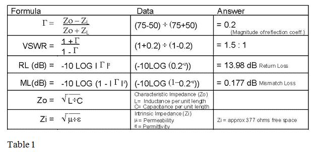
Table 1
From Table 1 above we see that the Mismatch loss is less than 0.2dB. Its also important to know that in this case the IF decoder receives a signal that has been translated to a much lower frequency with a lot of gain “upfront” in the LNB block. That gain does two things; sets the noise figure of the system at the LNB and provides isolation to downstream reflections.
The net effect is that even if some power is lost due to mismatch loss we have plenty of power to spare from the high gain amp upfront in the receiver chain. As for the reflected signal the high isolation of the LNB protects the system from being adversely affected. No worries!
** An analogous phenomenon occurs when ocean waves hit a vertical sea wall. Anyone who has witnessed such an event will recall seeing the wave come in, hit the wall and a new wave is born that travels back out to sea. Waves that hit a nice gradual beach dissipate with little or no reflected wave. You could say that a gradual beach has the characteristic impedance for typical surface waves on the ocean.